Read an NIfTI file
This is example to read a NIfTI file and apply TRANSFORMATIONS AND SMOOTHING , by using this example code you must be install package oro.nifti,AnalyzeFMRI: first.
Download a NIfTI file from Neurohacking_data repository
library(oro.nifti)


url <- "https://raw.githubusercontent.com/muschellij2/Neurohacking/master/Basic_Data_Manipulations/Kirby21/SUBJ0001-01-MPRAGE.nii.gz"
destfile <- "Output_3D_File.nii.gz"
name <- file.path(getwd(), destfile)
download.file(url, destfile,mode="wb") # NIfTI is binaryfile format
T1 <- readNIfTI(destfile)
As you see this file contain 22 images 512 x 512 pixels, one pixel using 16 bits
Visial an Slice an NIfTI file
image(T1,z=11,plot.type="single") 
Visualizing Log-Scale Histogram
im_hist<-hist(T1,plot=FALSE)
par(mar = c(5, 4, 4, 4) + 0.3)
col1=rgb(0,0,1,1/2)
plot(im_hist$mids,im_hist
$count,log="y",type='h',lwd=10, lend=2,
col=col1,xlab="Intensity Values",ylab="Count
(Log Scale)" ) 
Log-Scale Histogram with Linear Transfer Function
im_hist<-hist(T1,plot=FALSE)
par(mar = c(5, 4, 4, 4) + 0.3)
col1=rgb(0,0,1,1/2)
plot(im_hist$mids,im_hist
$count,log="y",type='h',lwd=10, lend=2,
col=col1,xlab="Intensity Values",ylab="Count
(Log Scale)" )
par(new = TRUE)
curve(x*1, axes = FALSE,xlab = "",ylab= "",
col=2, lwd=3)
axis(side=4,at = pretty(range(im_hist$mids))/
max(T1), labels=pretty(range(im_hist$mids)))
mtext("Original Intensity", side=4, line=2) 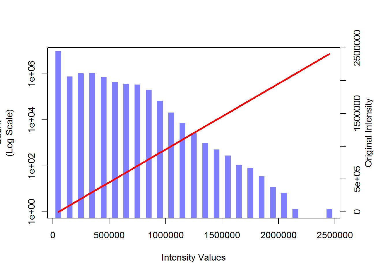
Plot the spline transfer function
#This defines a linear spline. Other definitions are possible
lin.sp<-function(x,knots,slope)
 {knots<-c(min(x),knots,max(x))
 slopeS<-slope[1]
 for(j in 2:length(slope)){slopeS<-c(slopeS,slope[j]-
sum(slopeS))}
 rvals<-numeric(length(x))
 for(i in 2:length(knots))
 {rvals<-ifelse(x>=knots[i-1], slopeS[i-1]*(x-knots[i-1])+rvals,
rvals)}
 return(rvals)}
#Define a spline with two knots and three slopes
knot.vals<-c(.3,.6)
slp.vals<-c(1,.5,.25)

im_hist<-hist(T1,plot=FALSE)
par(mar = c(5, 4, 4, 4) + 0.3)
col1=rgb(0,0,1,1/2)
plot(im_hist$mids,im_hist
$count,log="y",type='h',lwd=10, lend=2,
col=col1,xlab="Intensity Values",ylab="Count
(Log Scale)" )
par(new = TRUE)
curve(lin.sp(x,knot.vals,slp.vals),axes=FALSE,xlab="",ylab="",col=2,lwd=3)
axis(side=4,at = pretty(range(im_hist$mids))/
max(T1),labels=pretty(range(im_hist$mids)))
mtext("Transformed Intensity", side=4, line=2) 
Apply spline transfer function
trans_T1<-lin.sp(T1, knot.vals*max(T1), slp.vals)
image(T1,z=11,plot.type='single', main="Original Image")
image(trans_T1,z=11,plot.type='single',main="Transformed Image") 
Smoothing by GaussSmoothArray
library(AnalyzeFMRI)

smooth.T1 <- GaussSmoothArray(T1,voxdim=c(1,1,1),ksize=1,sigma=diag(3,3),mask=NULL,var.norm=FALSE)
orthographic(smooth.T1)